It’s been a couple of years since code4rena has introduced competitive audits into the smart contract security landscape, and it looks like audit contests are here to stay. In the meanwhile several other platforms have popped up with the same forumula.

Audit contests are simple. A project publishes a set of smart contracts that they would like to have audited, and promises a prize pool for security related findings. A contest is ran for a couple of weeks during which participants can submit their findings. The prize pool is then distributed based on the severity and uniqueness of the findings.

Audit contests have been tremendously successful in various ways. Aside from the many projects who’ve benefited from code contest reports, they’ve offered the opportunity to new security researchers to both train and prove themselves. Many solo auditors have started their careers by participating in audit contests.

One of the best parts for this post: All the results are available, and enough data has been accumulated to do some interesting analyses and answer some burning questions.

Let’s dive deep into some analytics of code contests data!

Questions

There are too many questions we could ask, in this post we’re going to focus on two main questions:

1. (coverage set) How many people do we actually need to find all the bugs?
2. (marginal value) How much value do we add with each additional participant? What’s the sweet spot?

Both these questions aim to give us some insight the economic efficiency of the audit contest model.

Data

We’ve pulled the last ~3 years of c4’s audit reports. So the results you’ll read in this post is primarily valid for code4rena. That said, alternative code contest platforms are similar so learnings from this data might still be applicable.

# block-description: we're data from c4 here. It contains all findings from all contests and each contest's reward distribution.

import math
import pandas
import pandas as pd
import mplcatppuccin
import matplotlib as mpl

mpl.style.use("mocha")

data = pandas.read_json('reports.json', typ='series')
normalised_base = pd.json_normalize(data)

# filter rows without findings ( not a list, empty list)

normalised_base = normalised_base[normalised_base['findings'].apply(lambda x: type(x) is list and len(x) > 0)]

Coverage Set

Let’s start with our first question: How much people do we actually need to find all the bugs? Or in other words, what’s the minimum amount of people from all participants that would’ve found all the bugs in the contest. This question will give us an initial insight into the efficiency of the contest model.

Not convinced?

An audit contest is at its core a resource allocation process. It employs incentives to get auditors to spend time on a project, and follows the core assumption “more people more findings”.

“more people more findings” is great, but what if we could find the same number of bugs with fewer people? How much money would we save? The smallest group of auditors that would find all bugs in an audit is what we will call the “coverage set”.

Example scenario: There are 100 participants, and we’d know we’d need just 10 (coverage set) to find all the bugs. We could skip the contest and just pay the 10 directly.

Even though it’s impossible to know a coverage set before a contest starts, the size of historical coverage sets are a good indicator of the optimal efficiency of a contest model.

Computing the Coverage Set

Computing the coverage set is easy! We can encode this problem as an optimisation problem and have a solver (cvxpy) find the solution for us:

# block-description: an algorithm to find the smallest coverage set of authors

import cvxpy as cp
import numpy as np

def smallest_coverage_set(set_of_sets):
    # Flatten and identify all unique elements across sets
    all_elements = set().union(*set_of_sets)
    element_to_index = {element: i for i, element in enumerate(all_elements)}
    n_elements = len(all_elements)

    # Create a binary variable for each element in the universal set
    x = cp.Variable(n_elements, boolean=True)

    # Constraints: Ensure at least one element from each set is selected
    constraints = []
    for s in set_of_sets:
        indices = [element_to_index[element] for element in s]
        constraints.append(cp.sum(x[indices]) >= 1)
    
    # Objective: Minimize the sum of binary variables (minimize the number of elements selected)
    objective = cp.Minimize(cp.sum(x))
    
    # Solve the problem
    problem = cp.Problem(objective, constraints)
    problem.solve() 
    
    # Retrieve the solution
    solution = np.round(x.value).astype(bool)
    selected_elements = [element for element, selected in zip(all_elements, solution) if selected]

    return selected_elements

# block-description: a simple utility function to extract the date from the title
def extract_date(title):
    # title format: yyyy-mm-title, take year and month and return datetime
    date = title.split('-')[:2]
    return pd.to_datetime('-'.join(date))

# block-description: measure coverage set analytics
result = []

for index, report in normalised_base.iterrows():
    if not 'findings' in report.keys():
        continue
    
    title = report['title']
    
    if type(report['findings']) is not list:
        continue
        
    findings =pd.json_normalize(report['findings'])

    if findings.empty:
        continue
        
    set_of_authors = findings[findings['authors'].notna()]
    set_of_authors = set_of_authors.explode('authors')
    set_of_authors = set_of_authors['authors'].unique()
    # set_of_authors.count()
    
    # people that have found issues on their own
    findings['author_count'] = findings['authors'].apply(lambda x: len(x) if x is not None else 0)

    single_author_findings = findings[findings['author_count'] == 1]
    unique_finders = set(single_author_findings.explode('authors')['authors'].unique())
    
    author_tgts = [ e for e in findings['authors'][findings['authors'].notna()].tolist() if e]
    if not author_tgts:
        continue
    smallest_coverage = smallest_coverage_set(author_tgts)
    
    result.append({'title': title, 'date': extract_date(title),'authors': set_of_authors, 'coverage_set': smallest_coverage})


result = pd.DataFrame(result)

# block-description: plot the number of authors, number of authors in coverage set and the percentage difference between the two
import matplotlib.pyplot as plt

result['n_authors'] = result['authors'].apply(lambda x: len(x))
result['n_coverage'] = result['coverage_set'].apply(lambda x: len(x))
result['coverage_diff'] = result['n_authors'] - result['n_coverage']
result['coverage_diff_pct'] = result['coverage_diff'] / result['n_authors'] * 100

# result['date'] = pd.to_datetime(result['date'])
# only select date, n_authors, n_coverage, coverage_diff
plot_data = result[['date', 'n_authors', 'n_coverage', 'coverage_diff', 'coverage_diff_pct']]

plot_data = plot_data.sort_values(by='date')
plot_data = plot_data.groupby('date').mean()

# remove last entry which is incomplete
plot_data = plot_data[:-1]

# human-readable labels for n_authors, n_coverage, coverage_diff
plot_data = plot_data.rename(columns={'n_authors': 'Number of Authors', 'n_coverage': 'Number of Authors in Coverage Set', 'coverage_diff_pct': 'Difference in Coverage Set %'})

from statsmodels.tsa.stattools import adfuller

print("""
The following are the results of the Augmented Dickey-Fuller test. The null hypothesis is that the data is non-stationary. If the p-value is less than 0.05 we reject the null hypothesis and conclude that the data is stationary.
""")
result = adfuller(plot_data['Number of Authors in Coverage Set'])
print(f'The number of authors in the coverage set is {"not" if result[1] > 0.05 else ""} stationary. p-value: {result[1]}')

result = adfuller(plot_data['Number of Authors'])
print(f'The number of authors is {"not" if result[1] > 0.05 else ""} stationary. p-value: {result[1]}')
if result[1] > 0.05:
    print(f"The number of authors is trending at a rate of {plot_data['Number of Authors'].diff().mean()} per month")

The following are the results of the Augmented Dickey-Fuller test. The null hypothesis is that the data is non-stationary. If the p-value is less than 0.05 we reject the null hypothesis and conclude that the data is stationary.

The number of authors in the coverage set is  stationary. p-value: 0.03455077312769427
The number of authors is not stationary. p-value: 0.2169667120943446
The number of authors is trending at a rate of 1.1870967741935483 per month

Coverage Results

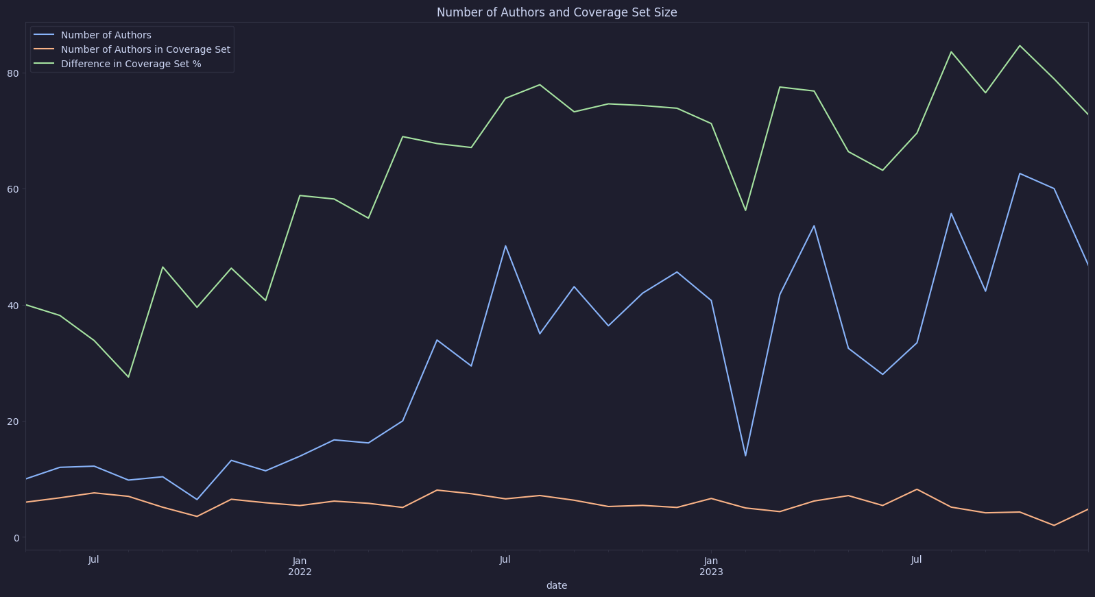
In the graph below we can compare the number of authors for each contest, and the size of the coverage set.

We can observe two things:

1. The number of authors is growing over time.
2. The number of authors in the coverage set staying the same.

This is very interesting! The number of authors h almost doubled, but our coverage set has stayed the same. This is a strong indication that there is an opportunity for more efficient resource allocation. Following the results of our dicky fuller test, we can see that these observations are statistically significant.

Note that we don’t account for authors that do not have issues attributed to themselves, this is often the case when authors only submit low severity or non-critical issues. This is an artifact of our dataset which doesn’t always attribute authorship for low and non-critical issues. Omitting low and non-critical issues from our analysis might actually be a good thing. It’s fairly trivial to come up with a unique non-critical issue. Because of this, we’re mostly interested in the coverage set for significant findings. Coincidentally, this is what the dataset provides us with!

plot_data.plot(y=['Number of Authors', 'Number of Authors in Coverage Set', 'Difference in Coverage Set %'], kind='line', figsize=(20,10))
plt.title('Number of Authors and Coverage Set Size')

Text(0.5, 1.0, 'Number of Authors and Coverage Set Size')

Ranking Participants

The following bit of code is using the Trueskill algorithm to build a ranking of all participants. Each individual contest is seen as a match where players are ranked based on their performance in the contest.

This ranking improves over the simple rewards based ranking present in many competitive audit leaderboards.

We’ll look more closely at ranking algorithms in a future post!

from analytics import AuditorRanking

auditor_ranking = AuditorRanking.build_trueskill_ranking(normalised_base)

Efficiency

Security engineers and project developers have a completely different perspective on security.

As a security engineer everything is about finding bugs, people should spend money on security because they don’t want bugs in their code. If there is a chance that there are still bugs in the code, then it’s worth spending money on security.

This is not how the rest of the world (should) think(s) about security. It’s often impossible to find all the bugs, and even if it was it would be so prohibitively expensive that the project would never be profitable. So instead people think about security in terms of risk.

$$risk = probability of a bug * cost of a bug$$

As more and more security measures ( like audits ) are implemented, the cost of reducing the probability of a bug increases, we observe diminishing returns. Aside from security, a team can also invest in alternative opportunities, with a projected return on investment. The cost of security is the opportunity cost of not investing in these alternative opportunities.

A development team will spend money on security until the opportunity cost of reducing the probability of a bug is equal to the risk of a bug.

Often the returns of security investments follow a logarithmic curve, and the optimum budget / sweet spot is often at what we call the “point of diminishing returns”. In this report, when we talk about the economic efficiency of a contest model, we’ll be speaking to the ability of the model to optimise risk reduction to cost.

Point of Diminishing Returns

Our data gives us simple data points: we know how much was spent and how much bugs were found. Or, in other words, the price (risk reduction / cost) of an audit contest.

Because we also know which bugs were found by which people, and how much money they made we can also compute the marginal value of each additional participant. With perfect foresight things would be easy, we’d just pick the smallest group of people that would find all the bugs. The coverage set!

However, not every participant is equal. How should we pick each additional participant?

Let’s start with an initial question. What’s our optimal case?

If we assume there exists an optimal participant selection algorithm, how many people would it pick? How would value increase as we add more people?

This question is simple! and answered by our previous analysis. We pick the coverage set! Beyond this group of people, we’re not adding any value.

Now we only need to find the most efficient crowd.

High Skill First

Let’s start with the most obvious approach: high skill first.

We’ll rank all participants by their skill level, and then add them to the contest one by one. We’ll measure the marginal value of each additional participant.

# block-description: utility function
def graph_cumulative_value_buckets(_data, _title, individual=True, value_reward=True):
    buckets = {
        10: [],
        20: [],
        40: [],
        80: [],
        150: []
    }
    
    def label_for_bucket(bucket):
        bucket_values = sorted(buckets.keys())
        idx = bucket_values.index(bucket)
        if idx == 0:
            return f"0 - {bucket}"
        elif idx > 0:
            return f"{bucket_values[idx - 1]} - {bucket}"
        else:
            return bucket
        
    for _, _report in _data.iterrows():
        if value_reward:
            _value_cumulative = _report['value_by_auditor_cumulative']
        else:
            _value_cumulative = _report['report_reward_by_auditor_cumulative']
            
        if len(_value_cumulative) > 150 and individual:
            plt.plot(_value_cumulative, label=len(_value_cumulative))
            continue
        for key in buckets.keys():
            if len(_value_cumulative) > key:
                continue
            buckets[key].append(_value_cumulative)
            break
    
    for key, values in buckets.items():
        plt.plot(mean_arrays(values), label=label_for_bucket(key))
    
    plt.legend()
    plt.title(_title)

# block-description: a method to measure marginal value
def skill_based_contribution_reward(reverse=False, exclude=False):
    _result = []
    
    def value_of_issue(issue):
        match issue['severity']:
            case 'High':
                return 9
            case 'Medium':
                return 3
            case _:
                return 1
        
    for index, report in normalised_base.iterrows():
        title = report['title']
        findings =pd.json_normalize(report['findings'])
        
        if findings.empty:
            continue
            
        set_of_authors = findings[findings['authors'].notna()]
        set_of_authors = set_of_authors.explode('authors')
        set_of_authors = set_of_authors['authors'].unique()
        
        # authors by skill level
        auditor_skill = [(auditor, auditor_ranking.get(auditor, 25)) for auditor in set_of_authors]
        
        # apologies for confusion reversing the table means not reversing skill
        auditor_skill = sorted(auditor_skill, key=lambda x: x[1], reverse=not reverse)
        
        total_value = 0
        
        skilled_auditors = [auditor for auditor, _ in auditor_skill]
        
        for _, finding in findings.iterrows():
            if finding['authors'] is None:
                continue
            for author in finding['authors']:
                if author in skilled_auditors:
                    total_value += value_of_issue(finding)
                    break
        
        report_value_by_auditor_cumulative = []
        report_value_by_auditor_cumulative_abs = []
        
        # total_reward = report['rewards'].sum()
        if isinstance(report['reward.rewards'], list):
            rewards = {
                reward['handle']: reward['awardTotal']
                for reward in report.get('reward.rewards', [])
            }
        else:
            rewards = {}
            
        total_reward = sum([float(v) for v in rewards.values()])
        
        report_reward_by_auditor_cumulative = []
        report_reward_by_auditor_cumulative_abs = []
        cumulative_counter = 0
        
        auditor_set = set()
        for auditor, skill in auditor_skill:
            if total_reward:
                cumulative_counter += float(rewards.get(auditor, 0))
                report_reward_by_auditor_cumulative.append(cumulative_counter / total_reward * 100)
                report_reward_by_auditor_cumulative_abs.append(rewards.get(auditor, 0))
            
            auditor_set.add(auditor)
            if len(auditor_set) == 1:
                continue
            
            # value of the set
            value = 0
            for _, finding in findings.iterrows():
                if finding['authors'] is None:
                    continue
                for author in finding['authors']:
                    if author not in auditor_set and exclude:
                        value += value_of_issue(finding)
                        break
                    if author in auditor_set and not exclude:
                        value += value_of_issue(finding)
                        break
                        
            percentage_value = (float(value) / total_value) * 100
            report_value_by_auditor_cumulative.append(percentage_value)
            report_value_by_auditor_cumulative_abs.append(value)
    
    
        _result.append({'title': title, 'value_by_auditor_cumulative': report_value_by_auditor_cumulative, 'value_by_auditor_cumulative_abs': report_value_by_auditor_cumulative_abs, 'total_value': total_value, 'report_reward_by_auditor_cumulative': report_reward_by_auditor_cumulative, 'report_reward_by_auditor_cumulative_abs': report_reward_by_auditor_cumulative_abs, 'total_reward': total_reward})
        
    _result = pd.DataFrame(_result)
    return _result

    

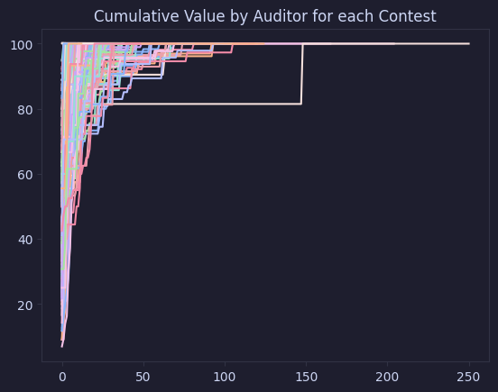
# block-description: plot the marginal value of each additional participant for each audit
value_auditor_skill = skill_based_contribution_reward()

for index, report in value_auditor_skill.iterrows():
    title = report['title']
    value_by_auditor_cumulative = report['value_by_auditor_cumulative']
    
    plt.plot(value_by_auditor_cumulative, label=title)

plt.title('Cumulative Value by Auditor for each Contest')

Text(0.5, 1.0, 'Cumulative Value by Auditor for each Contest')

# block-description: some utility funcs
from toolz import compose

# average the values
def mean_arrays(arrays):
    max_len = max(len(a) for a in arrays)
    mean_result = [0] * max_len
    
    for i in range(max_len):
        length_arrays = [a for a in arrays if i < len(a)]
        mean_result[i] = sum(a[i] for a in length_arrays) / float(len(length_arrays))
    
    return mean_result

def std_arrays(arrays):
    max_len = max(len(a) for a in arrays)
    std_result = [0] * max_len
    
    for i in range(max_len):
        length_arrays = [a for a in arrays if i < len(a)]
        std_result[i] = np.std([a[i] for a in length_arrays])
    
    return std_result

def add_arrays(base, other):
    return list(map(compose(sum, list), zip(base, other)))

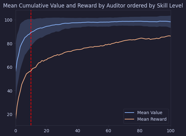
# block-description: plot the mean marginal value of adding participants
# add a vertical line at 10
plt.axvline(x=10, color='r', linestyle='--')

# stop after x == 100 bc data becomes too sparse
plt.xlim(0, 100)


mean_values = mean_arrays(value_auditor_skill['value_by_auditor_cumulative'])
mean_rewards = mean_arrays(value_auditor_skill['report_reward_by_auditor_cumulative'])

mean_values_plus_std = add_arrays(mean_values, std_arrays(value_auditor_skill['value_by_auditor_cumulative']))
mean_values_minus_std = add_arrays(mean_values, [-x for x in std_arrays(value_auditor_skill['value_by_auditor_cumulative'])])

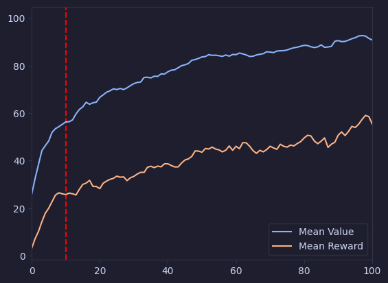
plt.plot(mean_values, label='Mean Value')
plt.plot(mean_rewards, label='Mean Reward')

plt.fill_between(range(len(mean_values)), mean_values_plus_std, mean_values_minus_std, alpha=0.2)

plt.legend()
plt.title("Mean Cumulative Value and Reward by Auditor ordered by Skill Level")

Text(0.5, 1.0, 'Mean Cumulative Value and Reward by Auditor ordered by Skill Level')

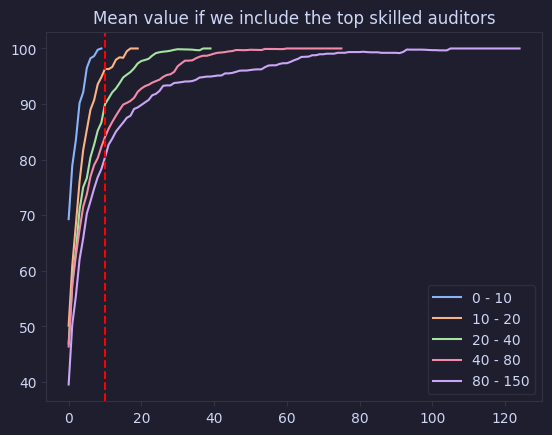
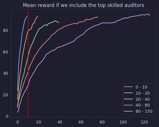
The following two graphs will explore the same data, but group the results in buckets based on the amount of participants in each contest. We’ll be using the following buckets: 0 - 10, 10 - 20, 20 - 40, 40 - 80, 80 - 150

This allows us to see if the size of the crowd affects anything, and better understand the data.

graph_cumulative_value_buckets(value_auditor_skill, "Mean value if we include the top skilled auditors", individual=False)
plt.axvline(x=10, color='r', linestyle='--')

<matplotlib.lines.Line2D at 0x2c1828f50>

graph_cumulative_value_buckets(value_auditor_skill, "Mean reward if we include the top skilled auditors", value_reward=False, individual=False)
plt.axvline(x=10, color='r', linestyle='--')

<matplotlib.lines.Line2D at 0x2c1776a50>

Discussion

Our graph clearly shows the logarithmic curve, adding more people to an audit involves the same diminishing returns we see with security controls in general. We also see that we’re investing quite a bit past the point of diminishing returns.

Interestingly we see that our curve changes as we have bigger contests! We see that as we have more people participating, we also see the point of diminishing returns delayed. Why this is the case will be the topic of a future post!

High Skill First (Exclude)

Let’s invert our analysis, and see what happens when we remove the high skilled auditors from the contest.

# block-description: plot the mean marginal value of adding participants
value_auditor_skill_exclude = skill_based_contribution_reward(exclude=True)
# add a vertical line at 10
plt.axvline(x=10, color='r', linestyle='--')
plt.axvline(x=3, color='g', linestyle='--')

# stop after x == 100 bc data becomes too sparse
plt.xlim(0, 80)

# we add 100 bc our loop skips it
mean_values = [100] + mean_arrays(value_auditor_skill_exclude['value_by_auditor_cumulative'])

mean_values_plus_std = add_arrays(mean_values, [0] + std_arrays(value_auditor_skill_exclude['value_by_auditor_cumulative']))
mean_values_minus_std = add_arrays(mean_values, [0] + [-x for x in std_arrays(value_auditor_skill_exclude['value_by_auditor_cumulative'])])

plt.plot(mean_values, label='Mean Value')

plt.fill_between(range(len(mean_values)), mean_values_plus_std, mean_values_minus_std, alpha=0.2)

plt.legend()
plt.title("Mean value if we exclude the top skilled auditors")

Text(0.5, 1.0, 'Mean value if we exclude the top skilled auditors')

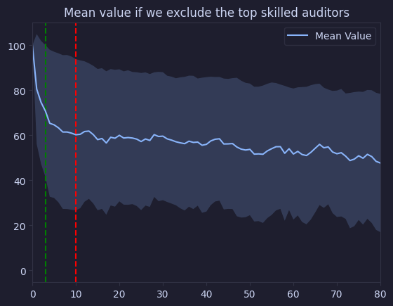
We see that removing the first skilled auditors has the most significant impact on audit quality. However, we also see that the value converges much faster than the previous graph.

The value stops decreasing as fast later on, let’s see if it is stationary:

# is value_auditor_skill_exclude value by auditor cumulative stationary after 20?
result = adfuller(mean_values[10:])
print(f'The value of the crowd is {"not" if result[1] > 0.05 else ""} stationary. p-value: {result[1]}')

The value of the crowd is not stationary. p-value: 0.9151256901698507

It is not! We must conclude that there seems consistent value in adding more participants, even after the top skilled auditors.

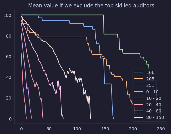
The following graph uses a bucket approach to visualise the data and confirms our previous findings. Removing the most skilled auditors has a significant impact on the value of the audit, but we see that the crowd still covers a decent bit of value.

# block-description: plot the mean marginal value of adding participants in buckets
graph_cumulative_value_buckets(value_auditor_skill_exclude, "Mean value if we exclude the top skilled auditors")

Low Skill First

Let’s invert our analysis!

Instead of picking from the “expensive” high skilled auditors, we’ll start with the low skilled auditors and add them to the contest one by one. We’ll measure the marginal value of each additional participant.

value_auditor_skill_reversed = skill_based_contribution_reward(reverse=True)

# add a vertical line at 10
plt.axvline(x=10, color='r', linestyle='--')

# stop after x == 100 bc data becomes too sparse
plt.xlim(0, 100)

mean_values = mean_arrays(value_auditor_skill_reversed['value_by_auditor_cumulative'])
mean_rewards = mean_arrays(value_auditor_skill_reversed['report_reward_by_auditor_cumulative'])
plt.plot(mean_values, label='Mean Value')
plt.plot(mean_rewards, label='Mean Reward')
plt.legend()

<matplotlib.legend.Legend at 0x2c1589a30>

graph_cumulative_value_buckets(value_auditor_skill_reversed, "Mean value if we include the low skilled auditors", individual=False)

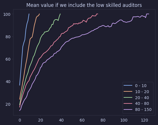
Low Skill First (Exclude)

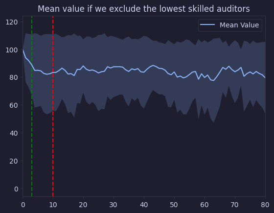
Similarly, we’ll invert our analysis, and see what happens when we remove the low skilled auditors from the contest.

# block-description: plot the mean marginal value of adding participants
value_auditor_skill_exclude = skill_based_contribution_reward(exclude=True, reverse=True)
# add a vertical line at 10
plt.axvline(x=10, color='r', linestyle='--')
plt.axvline(x=3, color='g', linestyle='--')

# stop after x == 100 bc data becomes too sparse
plt.xlim(0, 80)

# we add 100 bc our loop skips it
mean_values = [100] + mean_arrays(value_auditor_skill_exclude['value_by_auditor_cumulative'])

mean_values_plus_std = add_arrays(mean_values, [0] + std_arrays(value_auditor_skill_exclude['value_by_auditor_cumulative']))
mean_values_minus_std = add_arrays(mean_values, [0] + [-x for x in std_arrays(value_auditor_skill_exclude['value_by_auditor_cumulative'])])

plt.plot(mean_values, label='Mean Value')

plt.fill_between(range(len(mean_values)), mean_values_plus_std, mean_values_minus_std, alpha=0.2)

plt.legend()
plt.title("Mean value if we exclude the lowest skilled auditors")

Text(0.5, 1.0, 'Mean value if we exclude the lowest skilled auditors')

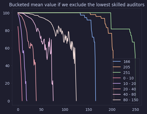
graph_cumulative_value_buckets(value_auditor_skill_exclude, "Bucketed mean value if we exclude the lowest skilled auditors")

Conclusion

We see something interesting!

1. There is value in adding more participants, even after the top skilled auditors.
2. Adding skilled auditors first is more efficient than adding low skilled auditors first.
3. C4’s model continues past the point of diminishing returns compared to an alternative selection method based on auditor skill.
4. Our strategy of picking high skilled auditors first allows us to get a better price (risk reduction / cost)

Limitations

We’re ordering the participants of a contest by relative skill. This means that the top ranking participant for any given contest could still have a relatively low skill level.

Furthermore, we’re using absolute positions. A participant at position 40 in an 80 participant contest, contributes to the index 40. Similarly, a participant at position 40 in a 40 participant contest also contributes to the index 40. This can confuse the interpretation of the graphs.

Point of Diminishing Returns within Universe

In our previous analysis we’ve investigated whether there is a point of diminishing returns within a single contest, which seems to be the case. This means that we could get a lot of the value of a contest by paying less.

The question now becomes: “could we get the same amount of value by paying less?”.

Our dataset tells us:

1. (theoretically) Yes, if we only pay the coverage set.
2. (in practice) Maybe, we’ll have to investigate this in a future post.

The Final Test before Mainnet

Audits and audit contests are sometimes used as a final check before going to mainnet.

Now, most security engineers will tell you that nothing will ever be perfect. There will always be bugs in the code. However, what does our data say?

To test whether this is a valid assessment we’ll investigate an interesting question:

If a top skilled auditor decides to participate in an audit how much unique value do they add?

Or in other words:

If they don’t participate, what’s the chance there is still something in the code?

This illustrates one mayor downside of competitive audits: that there is no actual guarantee that (all) (skilled) people will have a look at your audit.

Let’s find out!

# block-description: measure the average contribution of the top 10 auditors

top_50_auditors = sorted(auditor_ranking.keys(), key=lambda x: auditor_ranking[x], reverse=True)[:10]
auditor_pct_coverage = {auditor: [] for auditor in top_50_auditors}

def score(finding):
    match finding['severity']:
        case 'High':
            return 9
        case 'Medium':
            return 3
        case _:
            return 1
    
for index, report in normalised_base.iterrows():
    title = report['title']
    findings =pd.json_normalize(report['findings'])
    
    if findings.empty:
        continue
        
    
    total_value = sum(score(finding) for _, finding in findings.iterrows())
    
    for auditor in top_50_auditors:
        findings_by_auditor = findings[findings['authors'].apply(lambda x: auditor in x)]
        unique_findings_by_auditor =findings[findings['authors'].apply(lambda x: auditor in x and len(x) == 1)]
        
        auditor_score = sum(
            float(score(finding)) 
            for _, finding in unique_findings_by_auditor.iterrows()
        )
        if findings_by_auditor.empty:
            continue
        auditor_pct_coverage[auditor].append(auditor_score / total_value * 100.0)
    
    
coverages = []
coverage_means = []
for auditor, coverage in auditor_pct_coverage.items():
    coverages += coverage
    coverage_means.append(np.mean(coverage))
    
print(np.mean(coverages))

# test if mean is statistically significant from 0
from scipy.stats import ttest_1samp
res = ttest_1samp(coverages, 0)
print("t-statistic: ", res.statistic)
print(f"p-value: {res.pvalue:.20f}")
print(res.confidence_interval())

8.94375680426199
t-statistic:  9.617322706696772
p-value: 0.00000000000000000762
ConfidenceInterval(low=7.108369719533152, high=10.779143888990829)

👆 By joining a contest a top skilled auditor can expect to have unique findings in an audit.

Combined with our previous findings that more people are generally expected to find more bugs, we can conclude that security researchers are right.

Silver bullets do not exist, and we always expect there to be more bugs!

Limitations

The analysis provides some interesting insights into the contest model. However, it’s all too easy to have an overly optimistic / pessimistic interpretation of the results.

The analysis does not compare other models such as bug bounties or traditional audits to audit contests. As such it would be irresponsible to take these results and say “oh your money is better spent on XYZ”.

Furthermore, our analysis is also incomplete with regards to budget setting. Our results do not reflect on the effects that a higher / lower prize pool for competitive audits would have.

Finally, the definition of efficiency is easy to misinterpret. In our analysis we have looked at cost optimisation. One can also look at efficiency as value optimisation. In such a case one would look to increase the amount of bugs found for the same amount of money. This is something our analysis does not provide conclusions on.

In short, if you read this analysis and think it’s core message is “we should stop running audit contests” then you’ve missed the point.

Lastly, there are some practical limitations to the approach we’ve taken in this analysis:

Trueskill

We’re working with Trueskill with parameters that have only had limited tuning, and whether trueskill is an appropriate approach for evaluating auditor skill hasn’t been determined.

This means that the selection and performance of selected top auditors could potentially be different (likely higher) than they are in this analysis.

Even so, this yet unvalidated approach performed remarkably well in our analysis.

Value Modelling

Determining value of any given issue is a difficult task.

We’ve currently based our value model off the one used by code 4rena to determine the rewards for an audit, rating issues by their severity (high/medium/low/non-critical). Various factors are ignored in this model. There is no distinction between critical / non-critical, and potential financial impact is ignored.

As such we might see different results if we use a different value model.

Data

Unfortunately c4 doesn’t give us authors for all issues.

Future Work

Most of the limitations noted above provide opportunities for future work.

Value Modelling

It’s worth evaluating different models for the value of an audit, as the low / medium / high static scoring algorithm might be too simplistic.

For example, low, and medium findings, when fixed, might lead to significant improvements to a code base. On the other hand, we’ve anecdotally observed that low and medium findings are not of any interest to developers. As such their value might be overestimated by c4’s reward model.

Evaluating whether a value model provides appropriate incentives within the contest model itself is also an interesting avenue for future work.

Audits & Multiple Platforms

An obvious next step is to incorporate additional platforms’ data in this analysis, and to compare their behaviours.

Scheduling

Audit contests, solo audits, auditing firms, bug bounties, from the perspective of this analysis they’re all just different approaches to the “audit scheduling problem”.

This analysis provides an initial understanding of the balance between security research costs, and value. The initial evidence presented on this page suggests that selecting auditors by their skill level is an efficient way to get value. Future work should look at the correlation between value and a selection of auditors to see if there are more optimal approaches.

More!

Reach out to me if you have any ideas for future work! or if you’d like to collaborate!

twitter: @JoranHonig

Conclusion

These results lead us to two main conclusions:

1. c4’s reward model is not always perfectly economically efficient for risk reduction.
2. c4’s core assumption: “more people -> more findings” is sufficiently accurate.

Efficiency

In our analysis we have compared the incentives of projects getting their code audited, to the incentive model of audit contests and the ensuing results. Our main observation is that those incentives are not perfectly aligned. Instead, teams might get a better value to cost ratio using a different approach.

Interestingly we’ve already seen new models pop up that seem to follow some of the intuitions in this analysis. Paying some skilled auditors a set wage ( sherlock ) and running invite only contests ( code 4rena & more ) are just two examples. We also see many skilled contestants prove their skill during contests, to later focus on solo auditing.

The impact that skill has on the contributions of a participant has also been insightful. We must conclude that there are skilled auditors participating in c4 contests, and that their skill shows.

More People More Findings

We’ve seen that the size of the coverage set has remained stationary, which would suggest that more people might not mean more findings.

However, we’re yet unable to select the perfect group of auditors before a competition. In the realistic approaches we’ve applied in this post we did see that more people generally do lead to more findings. We’ve also seen that auditors of a very high skill-level are always expected to find unique findings in any audit they participate in.

So, in practice, we always expect that there are more bugs to be found!

All posts